Every commit has a risk, but can you quantify it? Teams go through a process to reduce risk, but whether it's a single line code change or vast refactor, the process is often the same. Quantifying the risk based on previous similar commits can help us decide whether it's worth taking some extra steps. Experienced teams have good intuition when deciding whether they've done enough, but cognitive biases can lead us astray. Stats can help with that, so in this article I share 4 methods of predicting the chance of a bug and compare the results.
The Data
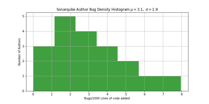
For this example I've run some analysis on SonarQube. Most developers will have come across this popular static analysis tool for finding bugs and security issues in code. It's an interesting repo because it appears to have a low defect rate (2 issues per 1000 lines of code added) and a small variance between developers. It looks like they eat their own dog food and deliver some very high quality code.
I extracted more than 20,0000 commits spanning the last 10 years, shuffled them, and split them 60/40 into a training and test set. For each commit I've extracted the author, a count of the lines of code added and tokenised the code for use in the machine learning methods later in the article.
A baseline: Linear Regression on Lines of Code Added
Bugs resides in code, so it follows that more code will increase the probability of more bugs. We can model this with linear regression using Numpy's polyfit function. This function derives the coefficients for least squares polynomial fit. We can specify the number of degrees to use and the coefficients can be passed to the poly1d function that returns a function we can use.
#linear regression
coeffs = np.polyfit(xtrain, ytrain, 1)
f1 = np.poly1d(coeffs)
print(f1)
0.001064 x + 0.2746
We can then use these functions to predict the probability of a bug in our test dataset and pass the results to a validator. For all these experiments I've used the BinaryAccuracy Validator in Keras for consistency.
validator = tf.keras.metrics.BinaryAccuracy()
validator.update_state(ytest, f1(xtest))
print('f1:',validator.result().numpy())
f1: 0.69960284
These methods give us 69-72% Accuracy. It's a good place to start
| Degree Polynomial | Function | Accuracy |
|---|---|---|
| 1st | 0.001064x + 0.2746 | 70% |
| 2nd | -2.424e-06x² + 0.002654x + 0.2112 | 71.6% |
| 3rd | 5.956e-09x³ - 9.318e-06x² + 0.004362x + 0.1732 | 72.2% |
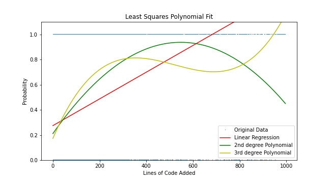
Here's the curves. It's interesting to see that on the 3rd Degree Polynomial there is a relatively flat section between 200-700 Lines of Code Added (LOCA) and then a rapid rise in risk. This might suggest that after 700 LOCA the commit becomes to large for us to safely comprehend and we miss problems.
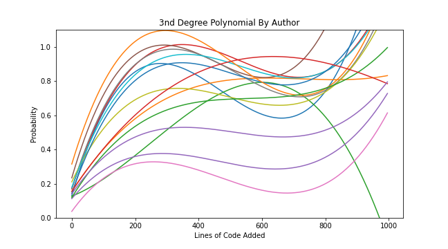
Developers are different: A Curve for each Committer
From the histogram at the beginning of this post we can see that although the variance between developers is relatively low at Sonar it's still significant, and if we factor this into a model we should see a more accurate result. The code below creates a function for every developer with over 100 commits and defaults to the general case for those with less.
authors = {}
for author, group in train_df.groupby('author'):
    if len(group) > 100:
        coeffs = np.polyfit(group.locadd, group.labels, 3)
        function = np.poly1d(coeffs)
        authors[author] = function

def auth_specific(author, locadd):
    author_func = authors.get(author)
    if author_func:
        return author_func(locadd)
    else:
        return f3(locadd)

test_predicted = []
for index, commit in test_df.iterrows():
    test_predicted.append(auth_specific(commit['author'], commit['locadd']))


validator = tf.keras.metrics.BinaryAccuracy()
validator.update_state(test_df['labels'], test_predicted)
print('auth_specific:',validator.result().numpy())
auth_specific: 0.7364434
In this case this strategy doesn't improve the overall accuracy of our predictions. In fact in most repos that I tried this on it performed worse than a single 3rd Degree Polynomial. The only exceptions are where there is a very large variance (>100:1) between the rate that developers create bugs.
| Degree Polynomial | Function | Accuracy |
|---|---|---|
| 3rd | Bespoke per committer | 70% |
A bit of AI: A basic Neural Network
So far we've only considered the size of the commit and the author but another factor we should consider is the type of code that was changed. Finding useful representations in unstructured code data is a job for machine learning, in this case we'll use Neural Networks (NN) and Natural Language Processing (NLP) techniques.
First up is a basic NLP Neural Network using word embeddings, a flatten and a single dense layer. The training sequences passed contain sequences for a string that starts with the author and then includes all the code in the commit.
from keras.models import Sequential
from keras.layers import Flatten, Dense, Embedding, Dropout


model = Sequential()
model.add(Embedding(len(data_sonar.tokenizer.word_index), 16, input_length=10000))
model.add(Flatten())
model.add(Dense(1, activation='sigmoid'))
model.summary()
model.compile(
    optimizer=tf.keras.optimizers.RMSprop(learning_rate=0.00001),
    loss='binary_crossentropy',
    metrics=[tf.keras.metrics.BinaryAccuracy()])
model.fit(data_sonar.train_sequences, data_sonar.train_labels,
    epochs=30,
    batch_size=8,
    validation_split=0.33)
model.evaluate(data_sonar.test_sequences, data_sonar.test_labels)
This gives us an accuracy of 73%. It's marginally the best yet. It's a great starting point for machine learning. Lets try something a bit more sophisticated.
A Bit More AI: A Convnet
Finally lets try a Convnet. Convnets or Convolutional Neural Networks are commonly used for image recognition but can but can perform well on text sequences. They work in a similar way to the neurons in our visual cortex by finding abstractions and passing these simpler representations to the next layer. It's possible that they may discover patterns in code that can increase the probability of a bug. Lets give it a try...
model = Sequential()
model.add(Embedding(len(data_sonar.tokenizer.word_index), 128, input_length=10000))
model.add(layers.Conv1D(32, 7, activation='relu'))
model.add(layers.MaxPool1D(5))
model.add(layers.Conv1D(32, 7, activation='relu'))
model.add(layers.GlobalMaxPool1D())
model.add(Dense(1, activation='sigmoid'))
model.summary()
model.compile(
    optimizer=tf.keras.optimizers.RMSprop(learning_rate=1e-4),
    loss='binary_crossentropy',
    metrics=[tf.keras.metrics.BinaryAccuracy()])
model.fit(data_sonar.train_sequences, data_sonar.train_labels,
    epochs=25,
    batch_size=8,
    validation_split=0.33)
model.evaluate(data_sonar.test_sequences, data_sonar.test_labels)
The result of this simple implementation on the SonarQube repo is again 73%. On other repos it shows an improvement over the simple Neural Network, with more tuning I'm expecting it to perform much better. The hard thing about machine learning is we don't know how this is working. Could it be considering code complexity, or perhaps it's doing little more than our polynomials?
Conclusion
To ensure these results can be replicated across other repos I've run the same tests on 3 other repos achieving similar results.
| Repo | Linear Regression | 2D Polynomial | 3D Polynomial | Author Bespoke Polynomial | Simple NN | Convnet |
|---|---|---|---|---|---|---|
| SonarQube | 69% | 71% | 72% | 70% | 73% | 73% |
| AspNet Core | 75% | 76% | 77% | 77% | 80% | 80% |
| Angular | 67% | 70% | 72% | 70% | 73% | 74% |
| React | 65% | 69% | 71% | 69% | 72% | 74% |
Bugs are hard to predict, but when we raise awareness of the risk before the damage is done, we can save a lot of pain later and increase development flow. Whilst these simple machine learning approaches don't offer large advantages over a statistical approach, they do seem to have the potential to recognise patterns of risky code which should significantly raise accuracy of predictions. If you're interested in exploring this further on your repos please get in touch or try ReviewML.